Profit and Loss Template in Excel: Build a 12-Month P&L (Free Download)

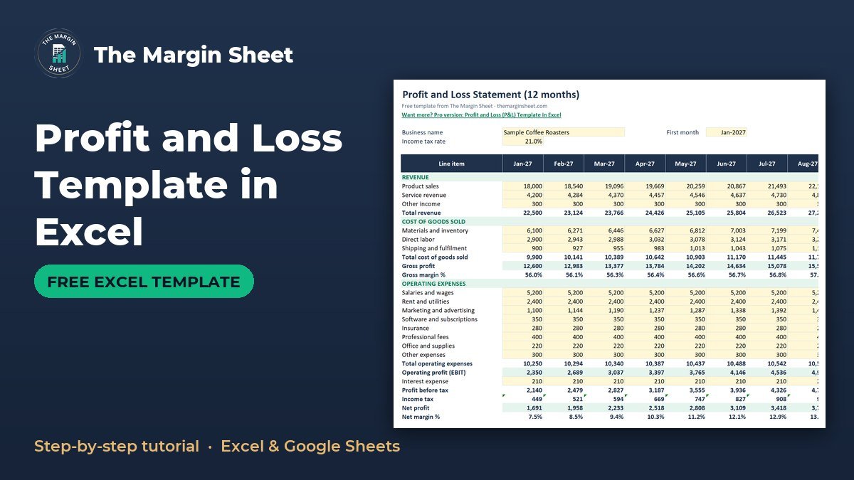
A profit and loss template in Excel lists your revenue, subtracts the cost of goods sold and operating expenses, and shows net profit for each month. To make one, you set up 12 month columns, add formulas for totals, gross profit, operating profit, tax and net profit, then type in your own figures. The free 12-Month Profit and Loss Template (Excel) is below, already built so you can follow along.

What this profit and loss statement in Excel does

A profit and loss statement, also called an income statement, shows whether your business made money over a period. This workbook covers 12 months on one sheet, with a Total column at the end. You type in the money coming in and going out, and the sheet works out gross profit, operating profit, tax and net profit for every month.

The file has two sheets: How to use and P&L. You enter the numbers on the P&L sheet and the formulas do the rest. A bar chart compares revenue and net profit by month, and net profit turns red when it is negative.

Who this income statement template is for

The sheet is written for people who run their own numbers and want a monthly picture without an accounting package. It fits these situations:

• A small business P&L for an owner who wants to see profit month by month.
• A freelancer or side business that needs to know what is left after costs and tax.
• Anyone preparing figures to discuss with a bookkeeper or adviser.
• A team lead who wants one clear page showing how revenue turns into net profit.

It is a planning and tracking tool. It does not replace professional bookkeeping, and the tax row is a simple rate applied to profit, not tax advice.

How the sheet is laid out

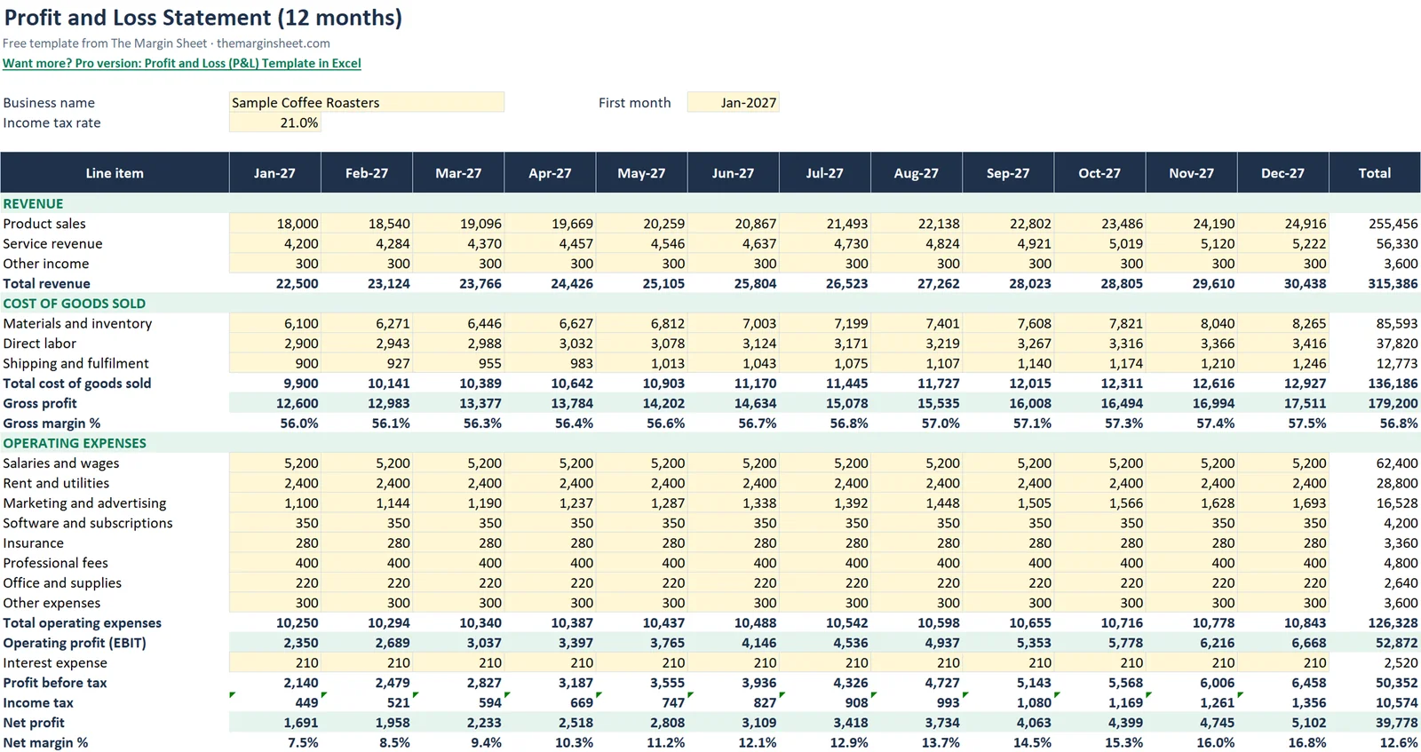
The sample business is Sample Coffee Roasters. The layout runs from top to bottom in the order a P&L is normally read, starting with sales and ending with net profit.

Section	Rows	What it holds
Inputs	B5, B6, G5	Business name, income tax rate, first month
Revenue	10-13	Product sales, Service revenue, Other income, Total revenue
Cost of goods sold	15-18	Materials and inventory, Direct labor, Shipping and fulfilment, Total COGS
Gross profit	19-20	Gross profit and gross margin %
Operating expenses	22-30	Eight expense lines and the total
Bottom line	31-36	EBIT, interest, tax, net profit, net margin %

Month headers sit in row 8, with Total in column N. Panes are frozen at B9, so the row labels and month names stay on screen while you scroll through the sheet.

Before you start: gather your figures

A P&L is only as good as the numbers you put in. Pull together your sales records, supplier invoices, payroll totals and bank or card statements for the month. Sort each item into one of the template lines before you type anything.

Decide early whether you will record income when you invoice a customer or when the money arrives, and then stay with that choice every month. Switching between the two methods makes month-to-month comparisons unreliable.

How to make a profit and loss statement in Excel, step by step

If you want to build it from scratch rather than use the download, work through these steps. Each one names the cells used in the template.

Step 1: Set up the inputs

Type your business name in B5. Enter your income tax rate in B6 (the sample uses 21%). Enter the first month in G5, for example Jan-2027.

These three cells drive the rest of the sheet. The month headers read from G5, and the tax row reads from B6, so you only change them in one place.

Step 2: Create the month headers

In B8 enter =G5. In C8 enter =EDATE(B8,1) and copy it across to M8. Put the word Total in N8. Format the dates as month and year.

EDATE moves a date forward by a set number of months, so each header is exactly one month after the one before it. That gives you 12 columns, B to M, with no typing of month names.

Step 3: Add revenue

List Product sales, Service revenue and Other income in rows 10 to 12. In row 13 enter =SUM(B10:B12) for Total revenue and copy it across to column M.

Step 4: Add cost of goods sold

Rows 15 to 17 hold Materials and inventory, Direct labor and Shipping and fulfilment. In row 18 enter =SUM(B15:B17) for Total COGS. These are the costs tied directly to making or delivering what you sell.

Step 5: Calculate gross profit and gross margin

In B19 enter =B13-B18. In B20 enter =IF(B13=0,0,B19/B13) and format it as a percentage. The IF stops a divide-by-zero error in a month with no revenue. For more on margin maths, see the profit margin formula guide for gross margin, markup and pricing.

Step 6: Add operating expenses

Rows 22 to 29 hold Salaries and wages, Rent and utilities, Marketing and advertising, Software and subscriptions, Insurance, Professional fees, Office and supplies, and Other expenses. In row 30 enter =SUM(B22:B29) and copy it across.

These are the overhead costs of running the business, whether or not you sold much that month.

Step 7: Work out operating profit

In B31 enter =B19-B30. This is operating profit, also called EBIT. It shows what the core business earned before interest and tax.

Step 8: Add interest, tax and net profit

Row 32 is an input row for interest expense. If you carry a loan, the loan amortization schedule in Excel shows the interest portion of each payment. Then use these formulas:

• B33: =B31-B32 for profit before tax
• B34: =MAX(0,B33*$B$6) for income tax, which gives no tax on a loss
• B35: =B33-B34 for net profit
• B36: =IF(B13=0,0,B35/B13) for net margin %

The $B$6 reference is locked with dollar signs, so it still points at the tax rate when you copy the formula across the other months.

Step 9: Fill the Total column and finish the formatting

In column N, use =SUM(B:M) style totals for each amount row, for example =SUM(B10:M10). Margin rows use the same formula as the monthly columns, applied to the totals, so the year margin is calculated from year totals and not averaged from the months.

Add conditional formatting so net profit turns red when it is below zero. Freeze panes at B9 so the labels and month headers stay visible as you scroll. Finally, add a bar chart that compares revenue and net profit by month.

Worked example with the sample figures

Sample Coffee Roasters has these results across the sample year:

Line	Year total
Total revenue	315,386
Gross profit	179,200
Gross margin %	56.8%
Net profit	39,778
Net margin %	12.6%

January net profit is 1,691. Gross margin shows how much of each sale is left after direct costs. Net margin shows what remains after operating expenses, interest and tax.

You can check the sample against the formulas. Revenue of 315,386 less gross profit of 179,200 means COGS for the year was 136,186. Gross profit divided by revenue gives the 56.8% gross margin, and net profit of 39,778 divided by the same revenue gives the 12.6% net margin.

The gap between 56.8% and 12.6% shows how much the overhead lines, interest and tax take. Those are the rows to check first if profit looks thin.

How to read your P&L once it is filled in

Start at the bottom and work upward. If net profit is red in a month, look at operating profit in row 31. If that is also negative, the problem sits in revenue, COGS or operating expenses, not in tax or interest.

Then compare gross margin across months. A falling gross margin in row 20 points to rising direct costs or lower prices. A steady gross margin with a falling net margin in row 36 points to overhead creeping up.

The bar chart helps here. Months where the revenue bar is tall but the net profit bar is short are the months worth a closer look line by line.

How to adapt it

• Rename the revenue, COGS and expense rows to match your business. Keep them inside the existing ranges so the SUM formulas still work.
• Change the tax rate in B6 to match your own rate. Check with a qualified adviser if you are unsure which rate applies.
• Change G5 to start the year in any month, such as a fiscal year start. The headers update through EDATE.
• Need more expense lines? Insert rows inside rows 22 to 29, not below row 29, so SUM(B22:B29) expands.
• Replace the sample business name in B5 with your own, and clear the sample figures from the input rows before you enter real ones.

A P&L shows profit, not cash. A sale you have invoiced but not collected counts as revenue, and a large purchase may not hit your costs the month you pay for it. For timing of money in and out, pair it with a cash flow forecast template in Excel.

A simple monthly routine

1. Enter the month’s revenue in rows 10 to 12.
2. Enter direct costs in rows 15 to 17.
3. Enter overhead in rows 22 to 29 and any interest in row 32.
4. Check that net profit in row 35 and the margins in rows 20 and 36 look reasonable.
5. Look at the bar chart and note any month that stands out.

Setting aside a fixed time each month keeps the sheet current, and a current sheet is far more useful than a perfect one that is three months behind.

Common mistakes

• Typing over formulas. Only the input rows (revenue, COGS, expenses and interest) should hold typed numbers.
• Mixing up COGS and operating expenses. Costs tied directly to making or delivering a product belong in COGS. Overhead belongs in operating expenses.
• Inserting rows outside the SUM range. New rows added below the last line of a section are not counted in the total.
• Deleting the tax rate reference. The income tax row uses $B$6, so keep that cell filled.
• Entering costs as negatives. The formulas subtract costs, so enter them as positive numbers.
• Averaging the monthly margins. The Total column calculates margin from the year totals, which is the correct figure. An average of 12 percentages gives a different answer.
• Leaving interest blank when you have a loan. Row 32 feeds profit before tax, so missing interest overstates profit.

Excel vs Google Sheets

The template is built in Excel, and every formula in it also works in Google Sheets. Upload the file to Google Drive and open it with Sheets.

Feature	Excel	Google Sheets
EDATE, SUM, IF, MAX	Works	Works
Freeze panes at B9	View, Freeze Panes	View, Freeze, then choose rows and columns
Red negative net profit	Conditional Formatting	Format, Conditional formatting
Bar chart	Insert, Chart	Insert, Chart

After importing, check that the month headers still display as dates and that the red formatting on net profit carried over. If a header shows a number such as 46388 instead of a date, change the cell format to month and year.

Where to go from here

The sheet works best when you update it monthly. Browse more options on the free templates page, or read the start here guide if you are new to spreadsheets. Paying down borrowing? The debt snowball spreadsheet helps plan it.

If you want a more extensive version, the Profit and Loss (P&L) Template in Excel is available as a paid option. You can also see other topics on the pro templates page.

Your next step: download the file, replace the sample figures in the revenue rows with last month’s actual numbers, and check that net profit in the first column looks right.

Education only. Not financial, tax or investment advice.