
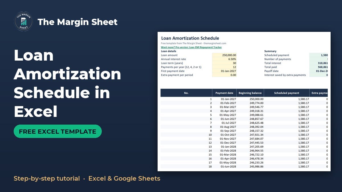
A loan amortization schedule in Excel lists every payment on a loan and splits each one into interest and principal. You build it by calculating the payment with the PMT function, then filling down a table where interest is the beginning balance times the periodic rate and principal is whatever is left of the payment. The free template is below, already set up with the formulas.
Free download
Loan Amortization Schedule (Excel)
Working formulas, sample data and a How to use sheet. Opens in Excel, or import it into Google Sheets.
What this template does and who it is for
The workbook has two sheets: How to use and Schedule. You type a loan amount, rate, term and start date into yellow input cells, and the Schedule sheet builds the full payment table, a summary and a line chart of the balance falling over time.
It suits anyone who wants to see what a loan really costs: a small-business owner checking an equipment loan, a freelancer looking at a vehicle loan, or a homeowner comparing what an extra payment would do. It handles monthly, quarterly, twice-yearly and yearly payments, and up to 480 payments.

This is an education tool, not financial advice. It shows the arithmetic of a loan with a fixed rate and regular payments, and it does not know your lender’s fees or rounding rules.
Why build an amortization schedule at all
A loan statement tells you the balance today. A schedule tells you the whole story: how much interest you will pay in total, when the loan ends, and how the split between interest and principal changes from the first payment to the last.
That view helps when you are comparing loan terms, planning cash for the coming year, or deciding whether paying a little extra each period is worth the effort. It also gives you something to check your lender’s figures against.
How the sheet is laid out
| Area | Cells | Purpose |
|---|---|---|
| Inputs (yellow) | B5:B10 | Loan amount, rate, term, payments per year, first payment date, extra payment |
| Summary | E5:E10 | Payment, number of payments, total interest, total paid, payoff date, interest saved |
| Schedule table | Header row 14, rows 15 to 494 | One row per payment, columns A to J |
The table columns are: A No., B Payment date, C Beginning balance, D Scheduled payment, E Extra payment, F Total payment, G Principal, H Interest, I Ending balance and J Cumulative interest. Keeping inputs, summary and table in separate blocks means you only ever type in the yellow cells.
Step-by-step: build the schedule
Step 1: Enter the inputs in B5:B10
Use these sample figures: B5 loan amount 250,000; B6 annual rate 6.5%; B7 term 30 years; B8 payments per year 12; B9 first payment date 01-Jan-2027; B10 extra payment per period 0. Set B8 as a dropdown list with the values 12, 4, 2 and 1 using Data Validation.
Shade the cells yellow so you remember they are the only ones meant for typing. Everything else in the sheet is a formula.
Step 2: Calculate the scheduled payment with PMT
In E5 enter =PMT(B6/B8,B7*B8,-B5). The rate is divided by payments per year and the term is multiplied by it, so the function works for any frequency. The minus sign in front of B5 makes the result a positive number. With the sample inputs it returns 1,580.17. This is the core of any PMT formula in Excel.
Step 3: Number the payments
In A15 enter 1. In A16 enter =IF(A15="","",IF(I15>0.005,A15+1,"")) and fill down to row 494. Numbering stops on its own once the ending balance reaches zero, so a shorter loan simply leaves blank rows below it.
Every other column checks column A first. If the number is blank, the row stays blank, which keeps the table tidy and keeps the chart and totals clean.
Step 4: Add the payment date
In B15 enter =IF(A15="","",EDATE($B$9,(A15-1)*12/$B$8)). EDATE moves the date forward by whole months, and the 12/$B$8 part sets the gap between payments: 1 month for monthly, 3 for quarterly, 6 for twice-yearly and 12 for yearly. Format the column as a date.
Step 5: Set the beginning balance
In C15 enter =$B$5. From C16 down, link to the previous row’s ending balance: =IF(A16="","",I15).
Step 6: Interest, payment, extra payment and principal
Fill these columns down, each wrapped in IF(A15="","",...):
- Interest in
H15:=C15*$B$6/$B$8 - Scheduled payment in
D15:=MIN($E$5,C15*(1+$B$6/$B$8)). The MIN means the last payment never overpays the loan. - Extra payment in
E15:=MAX(0,MIN($B$10,C15*(1+$B$6/$B$8)-D15)) - Total payment in
F15:=D15+E15 - Principal in
G15:=F15-H15
Principal is the total payment minus interest, so any extra payment lands entirely on principal.
Step 7: Ending balance and cumulative interest
In I15 enter =MAX(0,C15-G15). The MAX stops tiny rounding differences from showing a negative balance. Column J holds cumulative interest, which is a running total of column H: the interest paid so far, up to and including that row.
Step 8: Build the summary
E6number of payments:=MAX(A15:A494)E7total interest:=SUM(H15:H494)E8total paid: total interest plus the loan amountE9payoff date:=MAX(B15:B494)E10interest saved by extra payments:=MAX(0,E5*B7*B8-B5-E7)
Finally, select the ending balance column and insert a line chart so you can see the balance fall.
Worked example with the sample loan
With 250,000 at 6.5% over 30 years, paid monthly, the sheet shows these results:
| Result | Cell | Value |
|---|---|---|
| Scheduled payment | E5 | 1,580.17 |
| Number of payments | E6 | 360 |
| Total interest | E7 | 318,861.22 |
| Total paid | E8 | 568,861.22 |
| Payoff date | E9 | 01-Dec-2056 |
Check the first row to confirm your formulas. Interest is 250,000 x 6.5% / 12 = 1,354.17. Principal is 1,580.17 minus 1,354.17, which is 226.00. The ending balance is 249,774.00. If your first row matches, the rest of the table will follow.
Notice how little of the early payments goes to principal. That is why the total interest on this loan, 318,861.22, is more than the 250,000 borrowed.
Reading the result
The total paid in E8 is 568,861.22, which is the loan plus all the interest. Scroll down the table and you will see the interest column shrink while the principal column grows, because each payment reduces the balance that interest is charged on. The payment itself stays the same until the last row.
Using it as an extra payment calculator
Type an amount into B10, for example a fixed extra sum each period, and the schedule recalculates. The extra payment is added in column E and goes straight to principal, so the balance falls faster, the payoff date in E9 moves earlier and E6 drops below 360. The interest saved appears in E10.
Because column E is capped at what is still owed, the final payment adjusts itself and never overshoots. Compare the new total interest in E7 with the 318,861.22 baseline to see the difference.
Try small amounts first and watch how E6 and E9 respond. Before making extra payments on a real loan, check with your lender how they apply them, since some loans have conditions on early repayment.
How to adapt it
- Different frequency: pick 4, 2 or 1 in
B8. Dates, rate and payment all adjust. - Shorter or longer loans: change
B7. Rows beyond the final payment stay blank, and the table holds up to 480 payments. - Different start date: change
B9and every payment date shifts with it. - Business loans: use the payment and interest figures in a cash flow forecast template in Excel, and the interest total in your profit and loss template.
- Several debts: if you are deciding which balance to attack first, the debt snowball spreadsheet compares snowball and avalanche.
If the loan finances stock or equipment, the profit margin formula guide helps you check whether pricing covers the repayments.
Common mistakes
- Forgetting to divide the rate. Using 6.5% instead of
B6/B8inside PMT overstates the payment badly. - Mixing years and periods. The term must be multiplied by payments per year, as in
B7*B8. - Dropping the minus sign. Without
-B5, PMT returns a negative payment. - Missing dollar signs. References such as
$B$6must stay fixed when you fill down. If they slip, interest drifts wrong from row 16 onward. - Typing the rate as 6.5. Enter 6.5% or 0.065, or the sheet treats it as 650%.
- Stopping the fill at the wrong row. Fill to row 494 so loans of up to 480 payments fit.
- Expecting the lender’s exact figure. Lenders may round differently or add fees, so small differences from a statement are normal. Large ones are worth a question.
Excel vs Google Sheets
The template is built in Excel, but an amortization schedule in Google Sheets works too: upload the file to Drive and open it with Sheets. PMT and EDATE both exist in Google Sheets, so the formulas run unchanged.
| Item | Excel | Google Sheets |
|---|---|---|
| PMT and EDATE | Built in | Built in |
| Payments dropdown in B8 | Data Validation list | Check it still shows 12, 4, 2, 1 after import |
| Line chart | Insert, Chart | May need a quick restyle after import |
If you build the sheet from scratch in Google Sheets, use the same formulas from the steps above. Check the first row against the figures in the worked example, and the result will match.
More workbooks are on the free templates page, and the start here guide shows where to begin if you are new to spreadsheets.
Want a tracker instead?
If you would rather record payments as you make them in Google Sheets, the Loan EMI Repayment Tracker in Google Sheets is a paid option. Other paid sheets are listed by topic on the pro templates page.
Next step
Download the template, enter your own loan in B5:B10, and check the first row against your lender’s statement. Then try a small extra payment in B10 and see what it does to the payoff date.
Frequently asked questions
How do I create a loan amortization schedule in Excel?
Calculate the payment with =PMT(rate/payments per year, years*payments per year, -loan amount). Then build a table where interest is the beginning balance times the periodic rate, principal is the payment minus interest, and the ending balance is the beginning balance minus principal. Fill the rows down until the balance reaches zero.
What is the PMT formula in Excel for a loan?
The formula is =PMT(B6/B8,B7*B8,-B5), where B6 is the annual rate, B8 is payments per year, B7 is the term in years and B5 is the loan amount. For 250,000 at 6.5% over 30 years paid monthly, it returns 1,580.17.
How do I add extra payments to an amortization schedule?
Add an extra payment column that is capped at the remaining balance, and add it to the scheduled payment to get the total payment. In the template you type the amount in B10. The payoff date and total interest update automatically.
Can I use an amortization schedule in Google Sheets?
Yes. Upload the Excel file to Google Drive and open it with Google Sheets. PMT and EDATE both exist in Google Sheets, so the formulas keep working, though you may need to check the dropdown and chart.
Why is so much of my early payment interest?
Interest is calculated on the current balance, which is highest at the start. In the sample loan, the first payment of 1,580.17 includes 1,354.17 of interest and only 226.00 of principal.
Free download
Loan Amortization Schedule (Excel)
Working formulas, sample data and a How to use sheet. Opens in Excel, or import it into Google Sheets.
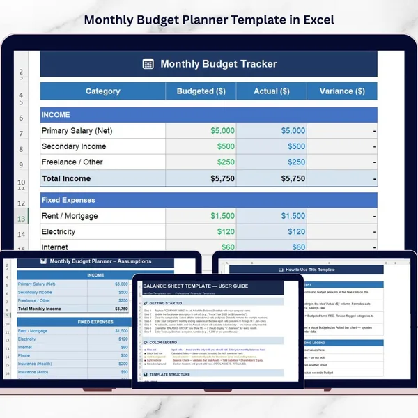
Want the finished version?
Monthly Budget Planner Template in Excel
Plan income and spending and compare budget against actual every month.
View the pro template
PK is the founder of PK: An Excel Expert and NextGenTemplates.com and a corporate trainer in Excel, VBA and Power BI. Since 2020 he and his team have built Excel and Google Sheets tutorials and templates for business users.
Education only. Not financial, tax or investment advice.