DCF Model in Excel: Step-by-Step Discounted Cash Flow (Free Template)

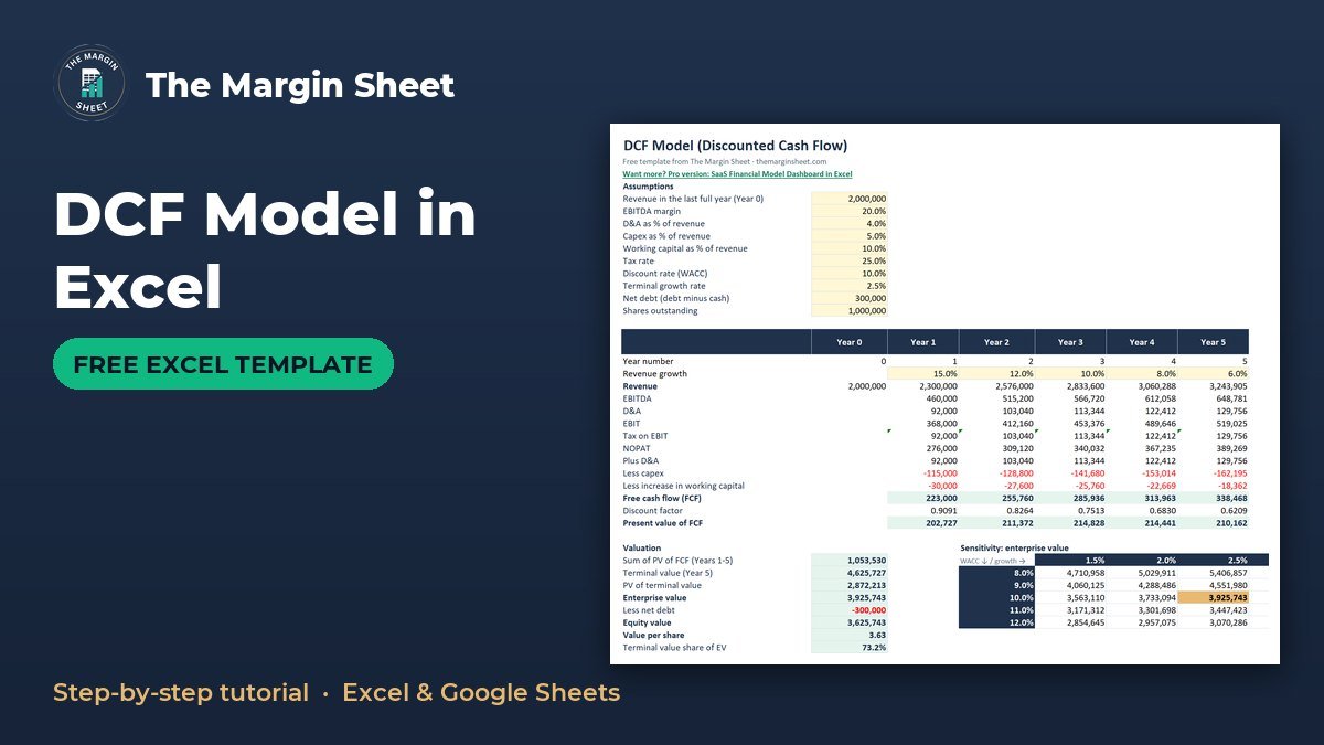
A DCF model in Excel estimates what a business is worth today by forecasting its free cash flow, discounting each year back at a required rate of return (WACC), and adding a terminal value for all the years after the forecast. You build it in seven steps: set assumptions, forecast revenue, work down to free cash flow, discount it, add terminal value, then subtract net debt to get equity value per share.

The free DCF Model Template (Excel) is below, with every formula already in place.

What this discounted cash flow Excel template does

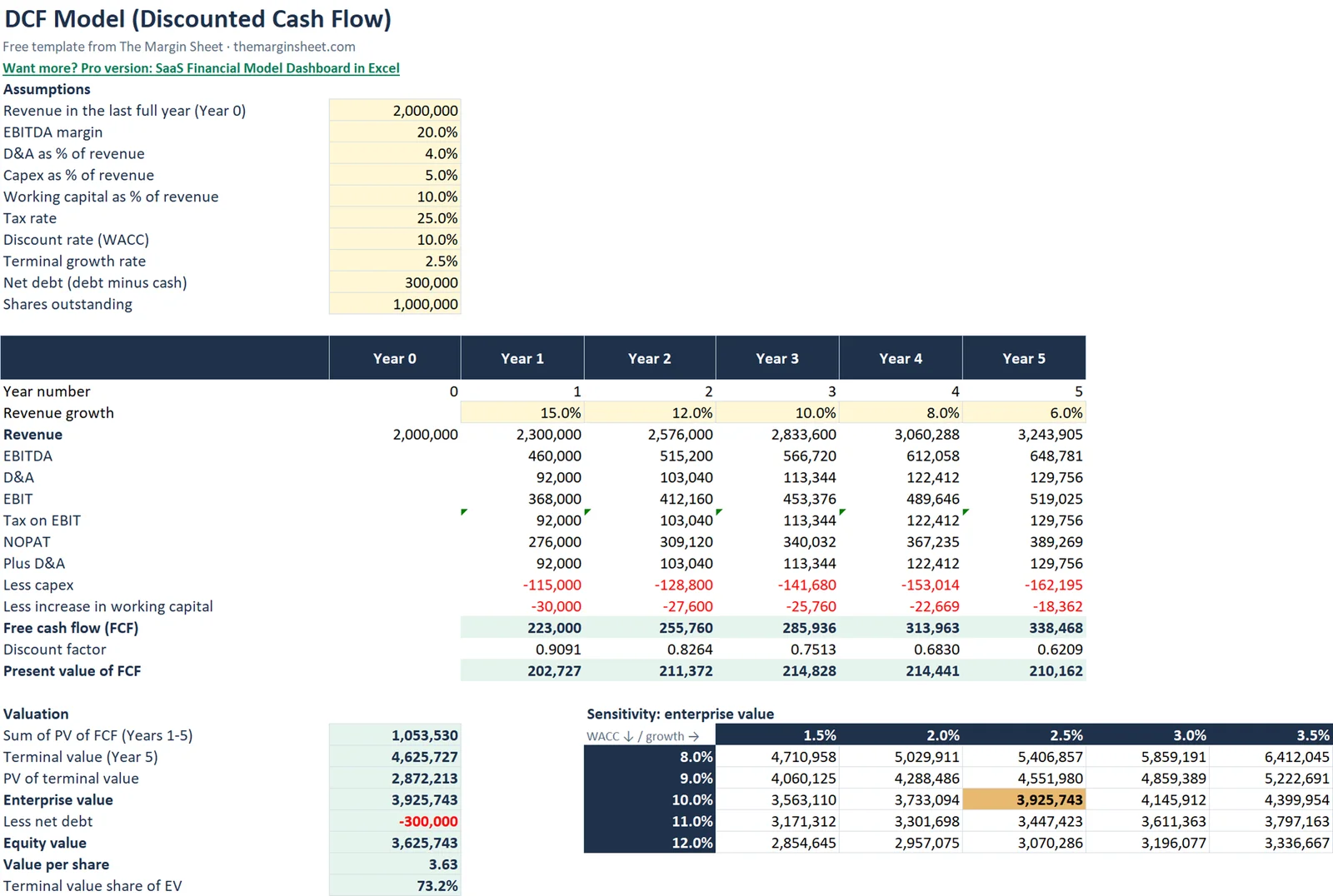
The template has two sheets: How to use and DCF. You type ten assumptions into B5:B14 and five growth rates into row 18. The sheet then builds a five-year forecast, discounts it, calculates terminal value and shows enterprise value, equity value and value per share.

It suits small-business owners valuing their own company, freelancers weighing up a business purchase, and students or analysts who want a clear model to learn from. This is education only, not investment advice.

What a DCF actually measures

A discounted cash flow values a business by the cash it is expected to produce, not by its profit on paper or by what similar companies sold for. Cash received in five years is worth less than cash received today, so each future amount is shrunk by a discount rate. In this template that rate is the WACC, set at 10% in the sample.

Because no forecast can run forever, the model forecasts five years in detail and then adds one lump sum, the terminal value, to stand for everything after Year 5. The total of those two pieces is enterprise value. Take away net debt and you have what belongs to the owners.

The same idea of shrinking future cash to today’s money sits behind the NPV formula in Excel, which is worth a look if discounting is new to you.

How to build a DCF model: step by step

Follow the steps below to rebuild the model from scratch, or use them to understand the finished template. Forecast columns run from B (Year 0) to G (Year 5), and row 17 holds the year number.

Step 1: Enter the assumptions in B5:B14

Put your inputs in a single block so you can change them without touching a formula. The template uses these sample values:

Assumption	Sample value
Year 0 revenue	2,000,000
EBITDA margin	20%
D&A (% of revenue)	4%
Capex (% of revenue)	5%
Working capital (% of revenue)	10%
Tax rate	25%
WACC	10%
Terminal growth	2.5%
Net debt	300,000
Shares outstanding	1,000,000

In the formulas, the EBITDA margin is $B$6, D&A is $B$7, capex is $B$8, working capital is $B$9, the tax rate is $B$10, WACC is $B$11 and terminal growth is B12. The dollar signs lock each reference so you can copy formulas across the row.

Step 2: Add the revenue growth inputs in row 18

Enter the growth rate for each forecast year in C18:G18: 15%, 12%, 10%, 8% and 6%. The rates step down each year, which is a common way to show a business maturing. Then forecast revenue in row 19. In Year 1 (column C) the formula is =B19*(1+C18), which gives 2,300,000. Copy it across to Year 5, which reaches 3,243,905.

Step 3: Work down from EBITDA to NOPAT

Each line below is shown for Year 1 in column C:

• EBITDA: =C19*$B$6 gives 460,000.
• D&A: =C19*$B$7 gives 92,000.
• EBIT: =C20-C21 gives 368,000.
• Tax on EBIT: =MAX(0,C22*$B$10) gives 92,000. The MAX stops the model from creating a tax credit if EBIT is negative.
• NOPAT: =C22-C23 gives 276,000.

NOPAT means net operating profit after tax. It is the profit from running the business, taxed as if there were no debt, so the cash flow stays separate from how the company is financed. Net debt is dealt with later.

Step 4: Apply the free cash flow formula

The free cash flow formula in this model is NOPAT + D&A – capex – increase in net working capital. Add back D&A because it is a non-cash cost. Then subtract two cash outflows:

• Capex: =-C19*$B$8 gives -115,000.
• Increase in working capital: =-(C19-B19)*$B$9 gives -30,000. It is 10% of the change in revenue, not of total revenue.

Year 1 free cash flow is 276,000 + 92,000 – 115,000 – 30,000 = 223,000. Year 5 free cash flow is 338,468. The growing business needs money tied up in equipment and working capital, which is why free cash flow sits well below EBITDA.

Step 5: Discount each year’s cash flow

The discount factor in Year 1 is =1/(1+$B$11)^C17. Multiply free cash flow by that factor to get the present value of each year, shown in row 30. The model uses end-of-year discounting, so Year 1 cash arrives at the end of year 1. In B33, =SUM(C30:G30) adds the five present values and gives 1,053,530.

Step 6: Calculate terminal value

The terminal value formula (Gordon growth) captures every year after Year 5. In B34 it is =G28*(1+B12)/(B11-B12), which gives 4,625,727. It takes the final-year free cash flow, grows it one more year at the terminal rate, and divides by the gap between WACC and that rate. Then B35 discounts it with =B34*G29, giving a present value of 2,872,213.

Terminal growth must stay below WACC. If it equals or exceeds WACC, the denominator is zero or negative and the result is meaningless.

Step 7: Reach equity value and value per share

Add the present value of the five years and the present value of terminal value. That gives an enterprise value of 3,925,743. Subtract net debt of 300,000 to get an equity value of 3,625,743. Divide by 1,000,000 shares and the value per share is 3.63.

Quick map of the Year 1 formulas

This table collects the Year 1 column in one place, so you can check your own build line by line.

Line	Year 1 formula	Year 1 result
Revenue	=B19*(1+C18)	2,300,000
EBITDA	=C19*$B$6	460,000
D&A	=C19*$B$7	92,000
EBIT	=C20-C21	368,000
Tax on EBIT	=MAX(0,C22*$B$10)	92,000
NOPAT	=C22-C23	276,000
Capex	=-C19*$B$8	-115,000
Increase in working capital	=-(C19-B19)*$B$9	-30,000
Free cash flow	NOPAT + D&A – capex – increase in NWC	223,000

Worked example with the sample figures

Here is the full valuation block in B33:B40, using the default inputs.

Item	Result
Sum of PV of FCF, Years 1-5	1,053,530
Terminal value	4,625,727
PV of terminal value	2,872,213
Enterprise value	3,925,743
Less net debt	300,000
Equity value	3,625,743
Value per share	3.63
Terminal value share of EV	73.2%

The last line matters. Terminal value makes up 73.2% of enterprise value, so most of the answer depends on two inputs: WACC and terminal growth. That is why the template includes a sensitivity grid.

Read the sensitivity grid in D33:I38

The grid tests WACC from 8% to 12% (rows) against terminal growth from 1.5% to 3.5% (columns). Each cell recalculates enterprise value with =SUMPRODUCT($C$28:$G$28/(1+$D34)^$C$17:$G$17)+$G$28*(1+E$33)/($D34-E$33)/(1+$D34)^5.

The base case (10% WACC, 2.5% growth) is highlighted gold and equals 3,925,743, matching the main valuation. The lowest value is 2,854,645 at 12% and 1.5%. The highest is 6,412,045 at 8% and 3.5%. That spread is large, so treat the result as a range rather than a single answer.

A practical way to use the grid is to pick the cell that matches your most cautious view and the cell that matches your most hopeful one. The distance between them shows how much your conclusion depends on judgment rather than arithmetic.

Sanity checks before you trust the result

• Check that the gold base case in the grid equals enterprise value in the valuation block. With the sample inputs both show 3,925,743.
• Confirm that terminal growth in B12 is lower than WACC in B11.
• Look at the terminal value share of EV. At 73.2% in the sample, the forecast years carry only about a quarter of the value, so be cautious about that share going higher.
• Compare Year 5 free cash flow of 338,468 with Year 1 at 223,000 and ask whether the growth path matches what you expect from the business.
• Make sure net debt is subtracted once, after enterprise value, and not inside the cash flows.

How to adapt the model

• Replace the Year 0 revenue and the five growth rates with your own figures.
• Change the EBITDA margin, capex and working capital percentages to match your business.
• Update net debt and shares outstanding. For a sole-owner business, you can set shares to 1 and read equity value directly.
• Adjust WACC and terminal growth, then check where the new base case sits in the grid.
• Change one input at a time and note the effect, so you learn which assumption moves the value most.

If you want to see how a growing balance behaves over time, the compound interest calculator in Excel shows the reverse of discounting. For other finance builds, browse the free templates page.

Common mistakes

• Terminal growth at or above WACC. The terminal value formula breaks. Keep growth below WACC.
• Overstating growth. A high growth rate in every year inflates the whole forecast.
• Forgetting the working capital change. Subtract only the increase, not the full balance.
• Ignoring net debt. Enterprise value is not what shareholders own. Subtract net debt first.
• Hard-coding numbers in formulas. Keep inputs in B5:B14 and row 18 so the grid and valuation update together.
• Trusting one number. With terminal value at 73.2% of EV, small input changes move the result a lot.
• Breaking the absolute references. If you drop the dollar signs in $B$6 or $B$11, copying a formula across the row points it at the wrong cell.

Excel vs Google Sheets notes

The template is built for Excel, and every formula used here also works in Google Sheets, including MAX, SUM and SUMPRODUCT. If you import it into Sheets, check that the gold highlight on the base case carried over, and confirm the grid still returns 3,925,743 at 10% and 2.5%.

Both programs use the same absolute reference style ($B$11), so copying formulas across the forecast behaves the same way. The start here guide explains how to open and copy the templates in either program.

Want a bigger model?

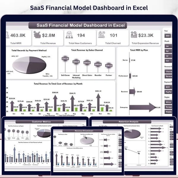
If you need a fuller forecast for a software business, the SaaS Financial Model Dashboard in Excel goes further than this five-year model. You can also see more options in the pro templates by topic.

Your next step

Download the template, keep the sample inputs and confirm you get a value per share of 3.63. Then replace the assumptions with your own and look at where your result sits in the sensitivity grid.

Education only. Not financial, tax or investment advice.