Compound Interest Calculator in Excel with Monthly Contributions (Free)

To build a compound interest calculator in Excel with monthly contributions, convert your annual rate into an equivalent monthly rate, then use the FV function to project the balance. With a 10,000 starting amount, 300 added each month, 7% a year and 20 years, the balance reaches about 196,665. The free template below does this for you and shows the yearly breakdown.

The free Compound Interest Calculator (Excel) template is below, followed by a full walkthrough of how it works.

What this calculator does and who it is for

The template projects how a lump sum and regular monthly deposits grow over time. You enter five inputs and it returns the final balance, the total you paid in, the interest earned, the effective annual rate and the years needed to double your money.

It suits freelancers planning a savings pot, small-business owners comparing options for spare cash, and anyone who wants to see how compounding behaves before trusting a rough guess. It is an illustration only. Returns are not guaranteed and nothing here is financial advice.

The workbook has two sheets: How to use and Calculator. The How to use sheet is a short guide to the inputs. Everything described below happens on the Calculator sheet.

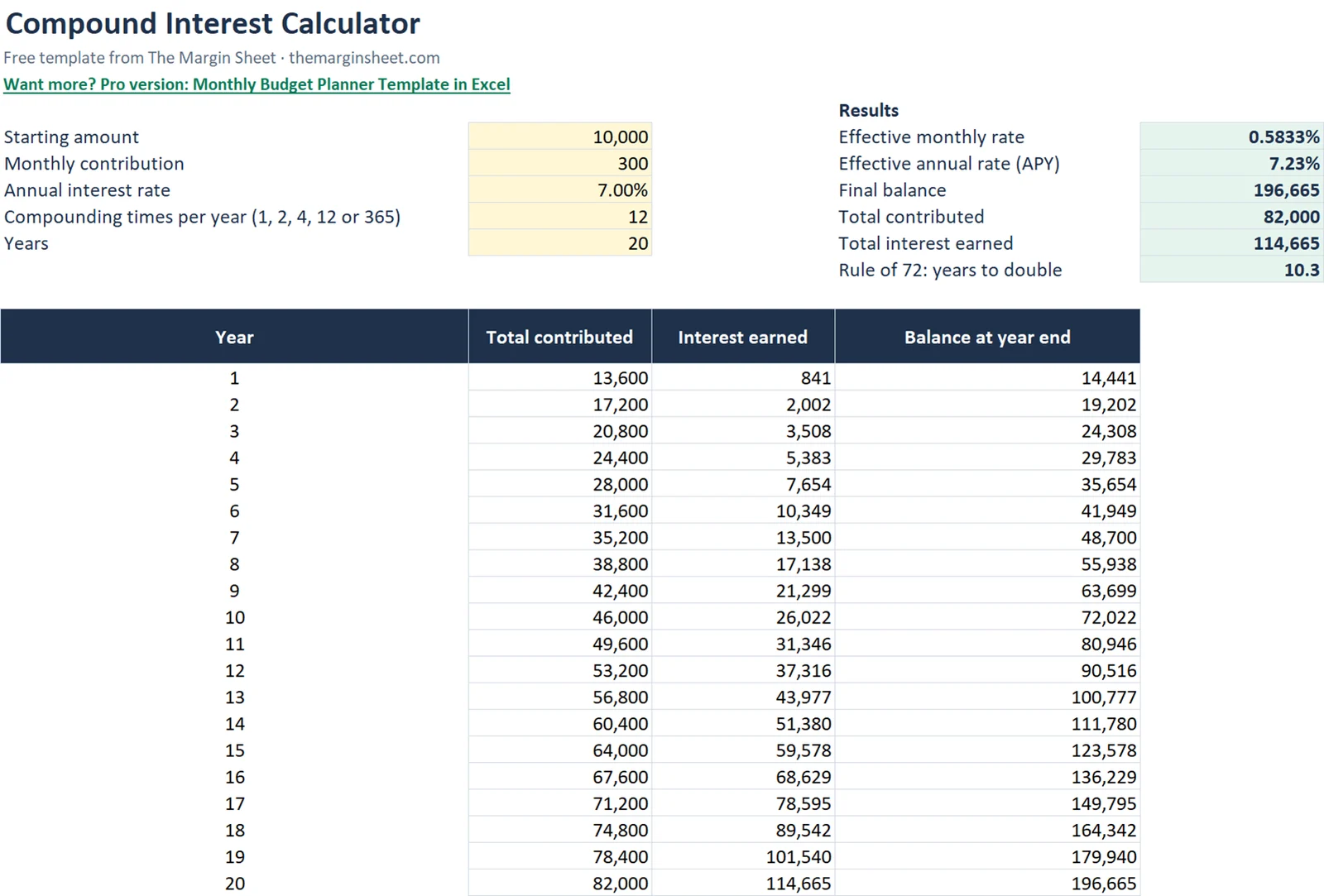
The top of the Calculator sheet holds the inputs on the left and the results on the right. Below them is a yearly table with a stacked column chart that splits each year’s balance into your contributions and the interest earned.

The inputs

The inputs sit in B5:B9. The sample values are in the table.

Cell	Input	Sample value
B5	Starting amount	10,000
B6	Monthly contribution	300
B7	Annual interest rate	7%
B8	Compounding times per year (dropdown: 1, 2, 4, 12 or 365)	12
B9	Years	20

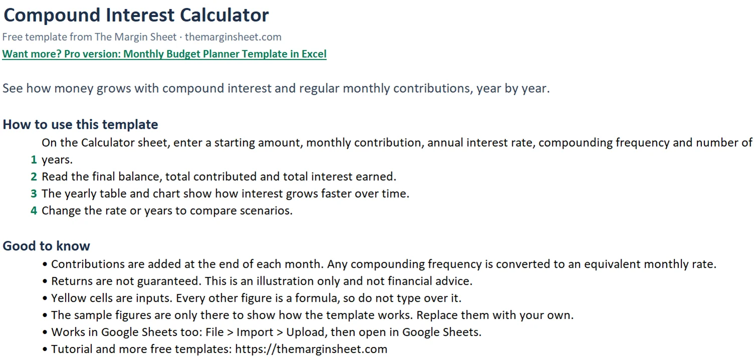
Contributions are assumed to be made at the end of each month. That timing matters for the result, so keep it in mind when you compare the output with a real account.

The results block

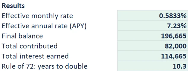
The results sit in E5:E10. Here is what each cell holds and the sample answer it gives.

Cell	Result	Formula	Sample value
E5	Effective monthly rate	=(1+B7/B8)^(B8/12)-1	0.5833%
E6	Effective annual rate (APY)	=(1+B7/B8)^B8-1	7.23%
E7	Final balance	=FV(E5,B9*12,-B6,-B5)	196,665
E8	Total contributed	=B5+B6*12*B9	82,000
E9	Total interest earned	=E7-E8	114,665
E10	Years to double (rule of 72)	=72/(B7*100)	10.3

How to calculate compound interest in Excel, step by step

Follow these steps on a blank sheet if you want to build the calculator yourself. If you downloaded the template, the formulas are already in place and you can use the steps to see what each one does.

Step 1: Set up the inputs

On a new sheet, type labels in column A and the values from the table above in B5:B9. Add a data validation list to B8 with the values 1, 2, 4, 12, 365 so you can switch compounding frequency from a dropdown without typing.

Format B7 as a percentage. Typing 7 into a cell that is not formatted as a percentage gives Excel the number 7, not 0.07, and every result will be wildly wrong.

Step 2: Convert the rate to an equivalent monthly rate

In E5 enter:

=(1+B7/B8)^(B8/12)-1

With the sample inputs this gives 0.5833%. This step matters because your deposits happen monthly, while the interest may compound daily, quarterly or yearly. Converting any frequency into an equivalent monthly rate lets the monthly contributions work with every option in the dropdown.

When B8 is 12, the exponent B8/12 equals 1 and the formula reduces to the annual rate divided by 12. For the other frequencies, the exponent adjusts the rate so that one month of growth matches what the chosen compounding would produce.

Step 3: Work out the effective annual rate

In E6 enter:

=(1+B7/B8)^B8-1

This is the APY. At 7% compounded monthly it comes to 7.23%. It is a handy figure for comparing accounts that compound at different frequencies, because a higher APY means more growth over one year from the same quoted rate.

Step 4: Calculate the final balance with the FV function

In E7 enter:

=FV(E5,B9*12,-B6,-B5)

The FV function in Excel takes the rate per period, the number of periods, the payment per period and the present value. Here the period is a month, so the rate is the monthly rate in E5 and the number of periods is B9*12. The payment is B6 and the present value is B5.

Both the payment and the present value are entered with a minus sign. Excel treats money you put in as outflow, so the negatives make the answer come back as a positive balance. The sample result is 196,665.

Step 5: Add total contributed and total interest

In E8 enter:

=B5+B6*12*B9

That returns 82,000: the 10,000 you started with plus 300 a month for 240 months (72,000). In E9 enter:

=E7-E8

This is the interest earned, 114,665 in the sample. It is the final balance minus everything you paid in.

Step 6: Estimate doubling time with the rule of 72

In E10 enter:

=72/(B7*100)

The rule of 72 is a quick mental shortcut: divide 72 by the annual rate as a whole number. At 7% it gives 10.3 years to double. It ignores monthly contributions, so treat it as a rough guide for a single lump sum.

Step 7: Build the yearly table

Put the headers in row 12: year, total contributed, balance at year end, interest earned. Fill rows 13 to 62 so the table can run up to 50 years. For a year number in column A, the formulas are:

• Total contributed: =$B$5+$B$6*12*A13
• Balance at year end: =FV($E$5,12*A13,-$B$6,-$B$5)
• Interest earned: balance minus contributed

The dollar signs lock the inputs so you can copy the formulas down. This is the core of the compound interest formula in Excel: the same FV call, with only the year changing.

Step 8: Add the chart

Select the contributions and interest columns and insert a stacked column chart. Each bar then shows how much of the balance came from your deposits and how much from interest. The interest part of the bar grows faster as the years go by.

Worked example with the sample figures

Using 10,000 to start, 300 a month, 7% compounded monthly for 20 years, the yearly table gives these checkpoints:

Year	Balance	Interest earned
1	14,441	841
10	72,022	26,022
20	196,665	114,665

In year 1 you have paid in 13,600 (10,000 plus 12 deposits of 300), so the 14,441 balance includes 841 of interest. By year 10 you have paid in 46,000 and the balance is 72,022, which means 26,022 came from interest.

The most interesting point is where interest overtakes your own money. In year 15 you have contributed 64,000 against 59,578 of interest. In year 16 you have contributed 67,600 against 68,629 of interest. From year 16 on, interest is the larger part of the growth.

At year 20 the totals match the results block: 82,000 contributed, 114,665 interest, 196,665 balance. If your own numbers do not line up between the yearly table and E7, one of the formulas has a wrong reference.

How to read the results

The final balance in E7 is a projection under fixed assumptions: a constant rate, deposits every month and no withdrawals. Real accounts rarely behave that neatly, so use the number to compare scenarios, not to predict an outcome.

The gap between E8 and E7 shows how much of the result depends on compounding rather than on your own deposits. The yearly table shows when that gap starts to widen quickly. The APY in E6 is useful when you compare two rates that compound at different frequencies.

How to adapt it

• Change B6 to 0 to see growth on a lump sum alone, and compare it with the rule of 72 result in E10.
• Switch the dropdown in B8 between 1, 2, 4, 12 and 365 to see how frequency changes the APY in E6.
• Extend B9 up to 50 years, which the yearly table supports.
• Set B5 to 0 to see what regular deposits alone build up to.
• Test a lower rate in B7 to see a more cautious scenario. Future returns are never guaranteed.

Change one input at a time and note how the result in E7 moves. That makes it clear whether the starting amount, the monthly deposit, the rate or the time period matters most for your case.

If you want to value future cash flows rather than grow savings, the NPV formula in Excel guide and the DCF model in Excel use similar time-value ideas in reverse. For a loan-side view of the same maths, see the mortgage calculator in Excel.

Common mistakes

• Wrong signs in FV. If the payment and starting amount are not negative, the balance shows as a negative number.
• Using the annual rate directly with monthly periods. Dividing 7% by 12 ignores the chosen compounding frequency. The template uses the equivalent monthly rate in E5 instead.
• Typing 7 instead of 7%. Format B7 as a percentage or the result will be far too large.
• Forgetting the timing. The template assumes deposits at the end of each month. Deposits at the start would give a slightly higher result.
• Breaking the locked references. Remove the dollar signs in the yearly table and the copied formulas point at the wrong cells.
• Mixing years and months. The number of periods in FV is B9*12 because the rate is monthly. Passing the years alone gives a far smaller balance.
• Treating the rule of 72 as exact. It is a shortcut for a lump sum. The full projection in E7 is the figure to rely on when you add monthly deposits.

Excel vs Google Sheets

The formulas work the same way in both programs. FV, the power operator and data validation lists all behave identically, so you can paste the formulas from this page into Google Sheets.

Task	Excel	Google Sheets
Final balance	=FV(E5,B9*12,-B6,-B5)	Same formula
Compounding dropdown	Data, Data Validation, List	Data, Data validation, Dropdown
Chart	Insert, Stacked Column	Insert, Chart, set type to stacked column

The template file is made for Excel, so open it in Excel for the cleanest result. If you work in Google Sheets, rebuild the chart after importing the file.

Next step

Download the template, enter your own starting amount and monthly deposit, and check the year when interest passes your contributions. Then change the compounding dropdown and the rate to see how sensitive the result is.

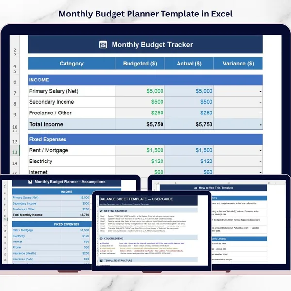
If you want to pair it with day-to-day money tracking, the Monthly Budget Planner Template in Excel is available as a paid option at NextGen Templates. You can find more sheets on the free templates page, or use the start here guide if you are new to the site.

This template is for education and illustration only. It is not financial advice.

Education only. Not financial, tax or investment advice.