

A mortgage calculator in Excel works out your monthly payment with the PMT function, then adds property tax, home insurance, HOA fees and PMI to give the full monthly cost. You enter the home price, down payment, rate and term, and the sheet returns the payment and a year-by-year balance table.
The free Mortgage Calculator (Excel) template is below, already built, so you can download it or follow the steps to make your own.
Free download
Mortgage Calculator (Excel)
Working formulas, sample data and a How to use sheet. Opens in Excel, or import it into Google Sheets.
What this mortgage calculator does and who it is for
The workbook has two sheets: How to use and Mortgage. The Mortgage sheet takes eight inputs and produces a PITI calculator style breakdown, plus HOA and PMI, so you see the real monthly figure and not just principal and interest.
PITI stands for principal, interest, taxes and insurance. Lenders and buyers use it because the loan payment alone understates what a home costs each month. This sheet adds HOA fees and PMI on top, so the total is closer to what leaves your bank account.
It suits first-time buyers comparing offers, people deciding how much down payment to put in, and anyone who wants to see how fast equity builds. It also helps landlords and freelancers who want a quick sanity check before talking to a lender. The numbers are estimates only and are not financial advice.
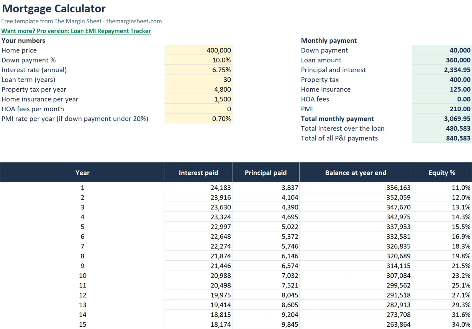
The inputs sit in B5:B12 on the left. The results sit in E5:E14 on the right. Below them, from row 17, is a yearly table that runs for up to 40 years, with a line chart of the loan balance.
Step-by-step: build the mortgage payment formula in Excel
Open a blank workbook, name one sheet Mortgage, and follow the steps in order. Put labels in column A for the inputs and in column D for the outputs, so you can read the sheet at a glance.
Step 1: Set up the inputs in B5:B12
On the Mortgage sheet, enter these values in column B, with labels in column A:
| Cell | Input | Sample value |
|---|---|---|
| B5 | Home price | 400,000 |
| B6 | Down payment (%) | 10% |
| B7 | Interest rate (yearly) | 6.75% |
| B8 | Term (years) | 30 |
| B9 | Property tax per year | 4,800 |
| B10 | Home insurance per year | 1,500 |
| B11 | HOA fees per month | 0 |
| B12 | PMI rate per year | 0.70% |
Format B6, B7 and B12 as percentages. PMI only applies when the down payment is under 20%, and the formula in step 5 handles that for you.
Step 2: Calculate the down payment and loan amount
In E5, enter =B5*B6. This gives the down payment in dollars: 40,000.
In E6, enter =B5-E5. This is the loan amount: 360,000. Every later formula points at E6, so the loan size flows through the whole sheet.
Step 3: Use the PMT function for principal and interest
In E7, enter =PMT(B7/12,B8*12,-E6). This is the core mortgage payment formula in Excel. The rate is divided by 12 for a monthly rate, the term is multiplied by 12 for the number of payments, and the loan amount is entered as a negative so the result shows as a positive payment.
With the sample inputs, the PMT function for the mortgage returns 2,334.95. That is the fixed monthly amount for principal and interest on a 360,000 loan at 6.75% over 30 years.
Step 4: Convert tax, insurance and HOA to monthly amounts
In E8, enter =B9/12 for property tax: 400.00.
In E9, enter =B10/12 for home insurance: 125.00.
In E10, enter =B11 for HOA, which is already monthly: 0.00.
Step 5: Add PMI with an IF test
In E11, enter =IF(B6<0.2,E6*B12/12,0). If the down payment is below 20%, PMI is the loan amount times the yearly PMI rate, divided by 12. Otherwise it is zero. In the sample, that gives 210.00.
Step 6: Total the monthly payment
In E12, enter =SUM(E7:E11). This is your total monthly payment: 3,069.95. It covers principal, interest, taxes, insurance, HOA and PMI.
Step 7: Work out total interest over the loan
In E13, enter =E7*B8*12-E6. That multiplies the monthly payment by the number of payments and subtracts the amount borrowed, which returns 480,583 of interest over the full term. E14 holds the total of all principal and interest payments: 840,583.
Build the mortgage amortization table in Excel
A yearly table shows where your money goes. Put the headers in row 17 and fill rows 18 to 57, which covers terms up to 40 years. Column A holds the year number (1, 2, 3 and so on). The columns are year, interest paid, principal paid, balance at year end and equity percentage.
Step 8: Interest paid each year
In B18, enter:
=-CUMIPMT($B$7/12,$B$8*12,$E$6,(A18-1)*12+1,A18*12,0)
Fill it down. The start and end arguments pick out the 12 payments that fall in each year. Year 1 shows 24,183 of interest.
Step 9: Principal paid each year
In C18, use the matching CUMPRINC formula with the same arguments, with a minus sign in front: =-CUMPRINC($B$7/12,$B$8*12,$E$6,(A18-1)*12+1,A18*12,0). Year 1 shows 3,837 of principal.
Step 10: Balance at year end
In D18, enter =MAX(0,$E$6-SUM($C$18:C18)). The anchored start of the range means each row adds up all principal paid so far. Year 1 ends at 356,163, and year 15 ends at 263,864. The MAX wrapper stops the balance from dropping below zero.
Step 11: Equity percentage
In E18, enter =($B$5-D18)/$B$5. Equity is 11.0% after year 1 and 34.0% after year 15. Select the balance column and insert a line chart to see the loan fall over time.
This mortgage amortization Excel table is yearly, not monthly, which keeps it short enough to read on one screen. Here are the checkpoints from the sample:
| Year | Interest paid | Principal paid | Balance at year end | Equity |
|---|---|---|---|---|
| 1 | 24,183 | 3,837 | 356,163 | 11.0% |
| 15 | – | – | 263,864 | 34.0% |
Worked example with the sample figures
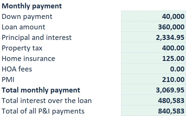
A 400,000 home with 10% down means a 360,000 loan at 6.75% over 30 years. The monthly breakdown looks like this:
| Item | Monthly amount |
|---|---|
| Principal and interest | 2,334.95 |
| Property tax | 400.00 |
| Home insurance | 125.00 |
| HOA | 0.00 |
| PMI | 210.00 |
| Total | 3,069.95 |
Over the loan you would pay 480,583 in interest, so the total of all principal and interest payments is 840,583 against a 360,000 loan. In year 1, 24,183 of your payments go to interest and only 3,837 reduce the balance.
That is why equity is just 11.0% after a year. The figure includes the 40,000 down payment, which is 10% of the price, so the first year of payments adds only about one more percentage point. By year 15 the balance has fallen to 263,864 and equity has reached 34.0%.
The PMI line is worth a second look. At 210.00 a month it is a visible part of the 3,069.95 total. Setting B6 to 20% removes it, and you can see the effect straight away in E11 and E12.
How to adapt the calculator
- Change B6 to 20% and E11 drops to 0, because the IF test no longer applies.
- Change B8 to 15 to compare a shorter term. The table adjusts, and rows past the term show a zero balance.
- Enter an HOA amount in B11 if your property has one.
- Try several interest rates in B7 to see how much each change moves E12.
- Replace B9 and B10 with quotes from your own area, since tax and insurance vary widely.
- Save a copy of the sheet for each property you are comparing, so the totals sit side by side.
If you want to see how savings grow instead of debt shrinking, the compound interest calculator in Excel uses a similar approach. For comparing a home purchase with other cash flows over time, see the guide to the NPV formula in Excel.
Common mistakes
- Forgetting to divide the rate by 12.
PMTneeds a monthly rate and a monthly number of periods. - Leaving the loan amount positive. Without the minus sign in
-E6, the payment comes out negative. - Typing 6.75 instead of 6.75%. Format B7 as a percentage or enter 0.0675.
- Entering yearly tax as monthly. B9 and B10 are yearly figures, and the sheet divides them by 12.
- Typing the down payment as a dollar amount. B6 is a percentage, and E5 multiplies it by the price.
- Treating PMI as permanent. The sheet keeps PMI for the whole loan for simplicity. In practice it is often removable at 20% equity, so your real payment may fall.
- Reading equity as market value. Equity here assumes the home keeps its purchase price.
- Breaking the anchors in the table. Keep the dollar signs in
$B$7,$B$8and$E$6so every row points at the same inputs.
Excel vs Google Sheets notes
The formulas work in both. PMT, CUMIPMT, CUMPRINC, IF, MAX and SUM are available in Excel and Google Sheets with the same arguments. If you upload the Excel file to Google Sheets, check the line chart and the percentage formats, since these are the items most likely to need a quick tidy.
The same logic applies to other loans such as car or personal loans: change the inputs and drop the tax and insurance lines. If you also send invoices from the same workbook habits, the invoice template for Google Sheets and Excel follows the same input-and-output layout.
Next step
Download the template, replace the sample figures with your own, and compare two or three scenarios by changing B6, B7 and B8. If you want more tools like this, browse the free templates page or the start here guide. For a broader valuation exercise, the DCF model in Excel is a good follow-up.
If you want a tracker for ongoing repayments, the Loan EMI Repayment Tracker in Google Sheets is a paid option. This calculator gives estimates only and is not financial advice.
Frequently asked questions
What is the mortgage payment formula in Excel?
Use =PMT(rate/12, years*12, -loan amount). With a 360,000 loan at 6.75% over 30 years, the template returns 2,334.95 per month for principal and interest. Taxes, insurance, HOA and PMI are added separately.
How do I add taxes, insurance and PMI to a mortgage calculation in Excel?
Divide yearly property tax and insurance by 12, add any monthly HOA, then add PMI with an IF test that applies it only when the down payment is under 20%. Sum these with the PMT result for the total. In the sample this is 3,069.95 per month.
How do I make a mortgage amortization schedule in Excel?
Use CUMIPMT for interest and CUMPRINC for principal over each year's 12 payments, then subtract cumulative principal from the loan amount for the balance. The template does this for up to 40 years. In year 1 it shows 24,183 of interest and 3,837 of principal.
Does the calculator work in Google Sheets?
Yes. PMT, CUMIPMT, CUMPRINC, IF, MAX and SUM work the same way in Google Sheets. After uploading the Excel file, check the chart and percentage formats.
Does the template remove PMI at 20% equity?
No. For simplicity it keeps PMI for the whole loan. In practice PMI is often removable at 20% equity, so your actual payment may drop over time.
Free download
Mortgage Calculator (Excel)
Working formulas, sample data and a How to use sheet. Opens in Excel, or import it into Google Sheets.
Want the finished version?
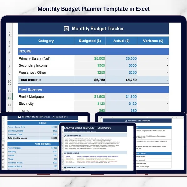
Monthly Budget Planner Template in Excel
Plan income and spending and compare budget against actual every month.
View the pro template
PK is the founder of PK: An Excel Expert and NextGenTemplates.com and a corporate trainer in Excel, VBA and Power BI. Since 2020 he and his team have built Excel and Google Sheets tutorials and templates for business users.
Education only. Not financial, tax or investment advice.