
To use the NPV formula in Excel, enter your discount rate, list each year’s cash flow with the initial investment as a negative number, and use =NPV(B5,B10:B19)+B9. Year 0 sits outside the NPV function because Excel treats the first value in the range as one period away. IRR comes from =IRR(B9:B19), and a positive NPV with an IRR above your discount rate points to the same decision.
The free NPV & IRR Calculator (Excel) is below, already built with a sample project.
Free download
NPV & IRR Calculator (Excel)
Working formulas, sample data and a How to use sheet. Opens in Excel, or import it into Google Sheets.
What this calculator does and who it is for
The workbook has two sheets, ‘How to use’ and ‘NPV’. You enter a discount rate and up to 11 cash flows (Year 0 to Year 10). It returns net present value, internal rate of return, profitability index, payback period and a plain-text accept or reject line.
It suits small-business owners weighing a purchase such as a machine or a fit-out, freelancers comparing equipment options, and busy professionals who need a quick capital budgeting check. It is for education and planning only, not financial advice.
If you need a full company valuation rather than a single project check, the DCF model in Excel covers that. NPV is the same idea at a smaller scale: discount future cash back to today and compare it with what you pay now.
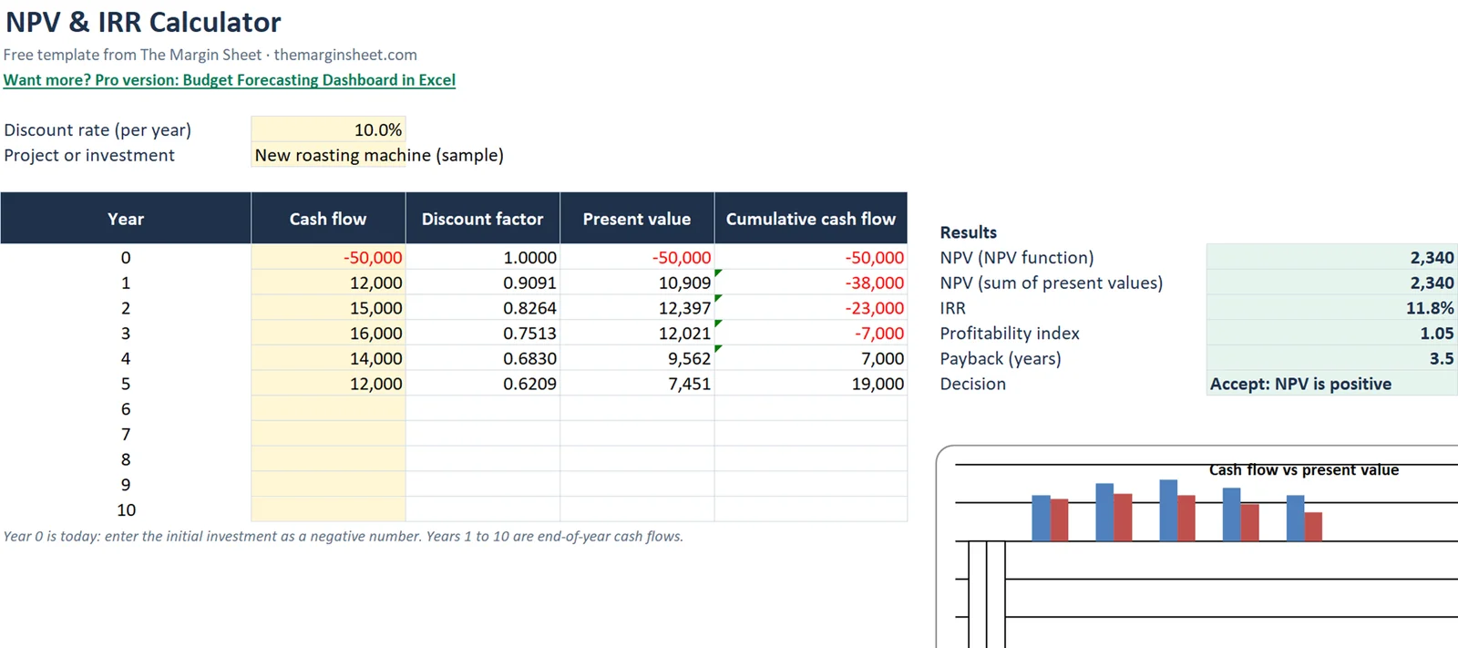
The sample project is called ‘New roasting machine’. It costs 50,000 up front and returns cash for five years, at a 10% discount rate. Every figure in this guide comes from that sample, so you can rebuild it cell by cell and check your numbers against ours.
What NPV and IRR actually measure
Net present value (NPV) answers one question: after charging the project for the return you require, how much value is left? A dollar received in five years is worth less than a dollar today, so each future cash flow is shrunk by a discount factor before it is added up. The discount rate is the return you demand, such as your cost of borrowing or a hurdle rate you set yourself.
Internal rate of return (IRR) turns the question around. Instead of choosing a rate and reading off a value, it finds the rate at which NPV is exactly zero. If that rate is higher than your discount rate, the project clears your bar.
The sheet also reports a profitability index and a payback period. Together these four numbers give you a rounded view of a single project without any macros or add-ins.
How to calculate NPV in Excel, step by step
Follow these steps on the ‘NPV’ sheet. If you would rather start from the finished file, download it above and use the steps as a guide to what each cell does.
Step 1: Enter the discount rate and project name
Type the project name in B6 and the discount rate in B5. The sample uses 10%. Use your own cost of capital or hurdle rate here. This single cell drives the discount factors, the NPV and the decision line, so changing it updates everything.
Step 2: List the cash flows
The table header is in row 8 and the data runs from row 9 to row 19. Column A holds the year (0 to 10) and column B holds the cash flow.
Enter the initial investment in B9 as -50,000, a negative number. In B10:B14 enter 12,000, 15,000, 16,000, 14,000 and 12,000. Leave Years 6 to 10 blank. Money going out is negative and money coming in is positive, which is what lets IRR work later.
Step 3: Add the discount factor
In C9 use this formula and copy it down to row 19:
=IF(B9="","",1/(1+$B$5)^A9)
The formula divides 1 by (1 + rate) raised to the year number. The IF keeps blank years empty, so unused rows do not clutter the table. The dollar signs on $B$5 lock the rate when you copy the formula down. At 10%, Year 1 gives 0.9091 and Year 5 gives 0.6209.
Step 4: Calculate present value
In D9 enter =B9*C9 and copy it down. Year 1 becomes 10,909 and Year 5 becomes 7,451. Each figure is what that year’s cash is worth today. Year 0 has a factor of 1, so the 50,000 outflow stays at full size.
Step 5: Track cumulative cash flow
In E9 enter =SUM($B$9:B9) and copy it down. The first six values are -50,000, -38,000, -23,000, -7,000, 7,000 and 19,000. The start of the range is locked while the end moves, so each row adds one more year. This column drives the payback period.
Step 6: Use the NPV function
In H9 enter:
=NPV(B5,B10:B19)+B9
The result is 2,340. The function discounts Year 1 onward, and Year 0 is added afterward because it happens today and needs no discounting. The range stops at row 19, so Years 6 to 10 are ready if you fill them in later.
Step 7: Cross-check with the sum of present values
In H10 enter =SUM(D9:D19). It also returns 2,340. Two methods giving the same answer is a quick proof that your range and discount rate are correct. If the two numbers differ, the usual cause is Year 0 placed inside the NPV function.
Step 8: Add the IRR formula
The IRR formula in Excel is:
=IFERROR(IRR(B9:B19),"No IRR")
It returns 11.8%. Notice that the range starts at B9, so the negative investment is included. IRR needs at least one negative and one positive value. The IFERROR shows “No IRR” when Excel cannot find a rate, for example if every value is positive.
Step 9: Add the profitability index
In H12 the profitability index is =SUM(D10:D19)/-B9, which gives 1.05. It divides the present value of the future cash by the amount invested. A result above 1 means you get back more in today’s money than you put in.
Step 10: Add payback period and a decision
Payback period in Excel is 3.5 years for the sample. Cumulative cash turns positive in Year 4, and the template finds that row with MATCH on the first non-negative cumulative value. The sum is 3 + 7,000/14,000: three full years, then half of Year 4’s 14,000 to clear the remaining 7,000.
The decision cell uses =IF(H9>0,"Accept: NPV is positive",...), so the sheet states the result in words next to the numbers.
Worked example with the sample figures
With a 10% discount rate and the cash flows above, the sheet produces these results:
| Measure | Result | Cell |
|---|---|---|
| NPV (function) | 2,340 | H9 |
| NPV (sum of present values) | 2,340 | H10 |
| IRR | 11.8% | H11 |
| Profitability index | 1.05 | H12 |
| Payback period | 3.5 years | H13 |
The roasting machine adds 2,340 of value in today’s money after meeting the 10% required return. The IRR of 11.8% is above 10%, so the two measures agree, and the decision line reads “Accept: NPV is positive”.
The profitability index of 1.05 says each unit invested returns 1.05 in present value. The cash is recovered during Year 4, when the cumulative column moves from -7,000 to 7,000.
The margin is thin. The machine returns 69,000 in plain cash over five years against 50,000 invested, but discounting trims the later years, which is why the NPV is a modest 2,340 and not something closer to the cash total. Seeing that gap is the main reason to use NPV and not a simple sum.
NPV vs IRR: which should you trust?
NPV gives an amount of value created. IRR gives a rate. When one project is judged alone, both usually lead to the same answer: a positive NPV means the IRR is above the discount rate, as in the sample.
When you compare projects, look at NPV first, because it shows the size of the gain. IRR can mislead when projects differ in scale or timing, since a small project can show a high rate and still add little value in absolute terms.
Payback tells you how fast you get your money back but ignores cash after that point, so treat it as a side check on risk and liquidity. The profitability index is useful when you have limited money and need to rank options by value per unit invested.
How to adapt the calculator
- Change
B5to test other discount rates. Higher rates shrink the present value of later years, so NPV falls as the rate rises. - Overwrite the cash flows in
B10:B19with your own forecasts. Use negative numbers for years with net outflows. - Fill in Years 6 to 10 if your project lasts longer. The formulas already cover those rows.
- Change the project name in
B6and save a copy per option, so you can compare a second machine or fit-out side by side. - Check the sign of every input. If the initial investment is not negative, IRR and the profitability index will not make sense.
The chart compares cash flow with present value in bars, so you can see how discounting reduces later years. The gap between the two bars grows as the years go on.
If your cash flows come from a loan or property, the mortgage calculator in Excel shows how to build the payment side. For growth over time rather than a project decision, try the compound interest calculator.
Common mistakes
- Including Year 0 inside NPV. This is the most common error.
=NPV(B5,B9:B19)discounts the initial investment by a full year and overstates the result. - Entering the investment as a positive number. It must be negative, or IRR cannot find a rate.
- Mixing a monthly rate with annual cash flows. Keep the periods consistent: annual rate with yearly flows, monthly rate with monthly flows.
- Leaving a zero in unused years instead of a blank. The discount factor formula checks for blanks, so a zero produces a row you did not intend.
- Starting the IRR range at
B10. IRR needs the negative Year 0 value in the range. - Ignoring the timing assumption. The template treats cash flows as arriving at the end of each year. For exact dates, use XNPV and XIRR.
- Trusting one result alone. Compare the function result with the sum of present values in
H10before you act on it.
Excel vs Google Sheets
Both programs share the same functions here. NPV, IRR, IFERROR, MATCH and SUM behave the same way, so the formulas paste across without edits. The same rule about Year 0 applies in both, so keep the initial investment outside the NPV range.
The template is built in Excel, but you can upload the file to Google Sheets and it should calculate normally. The chart may need a quick check after import, because chart formatting does not always carry over exactly.
XNPV and XIRR exist in both as well, which helps when payments fall on specific dates. If you are new to the site, the start here guide explains how the templates are organized and how to copy them into your own account.
Going further
Once the sample works, replace the cash flows with a forecast from your own business. If you want a structured place to build those forecasts, the Pro option is the Budget Forecasting Dashboard in Excel. You can also browse more free templates.
Next step: download the file, replace the sample cash flows with one real project, and check that both NPV methods match before you rely on the result.
Frequently asked questions
What is the NPV formula in Excel?
Use =NPV(rate, future cash flows)+initial investment. In the template that is =NPV(B5,B10:B19)+B9, which returns 2,340 for the sample project. Year 0 is added outside the function.
Why is Excel's NPV function wrong when I include Year 0?
Excel's NPV treats the first value in the range as one period away. Including the initial investment there discounts it by a full year. Add it after the function instead.
How do I calculate IRR in Excel?
Use =IRR(B9:B19) on the full range of cash flows, including the negative Year 0 value. The sample project returns 11.8%. Wrapping it in IFERROR shows a message if no IRR exists.
What is the difference between NPV and IRR?
NPV is the value created in today's money at your chosen discount rate. IRR is the rate at which NPV equals zero. If IRR is above your discount rate, NPV is positive, as in the sample (11.8% vs 10%).
How do I find the payback period in Excel?
Build a cumulative cash flow column with =SUM($B$9:B9) and find the first year it turns non-negative. In the sample that is Year 4, giving 3.5 years (3 + 7,000/14,000).
Free download
NPV & IRR Calculator (Excel)
Working formulas, sample data and a How to use sheet. Opens in Excel, or import it into Google Sheets.
Want the finished version?
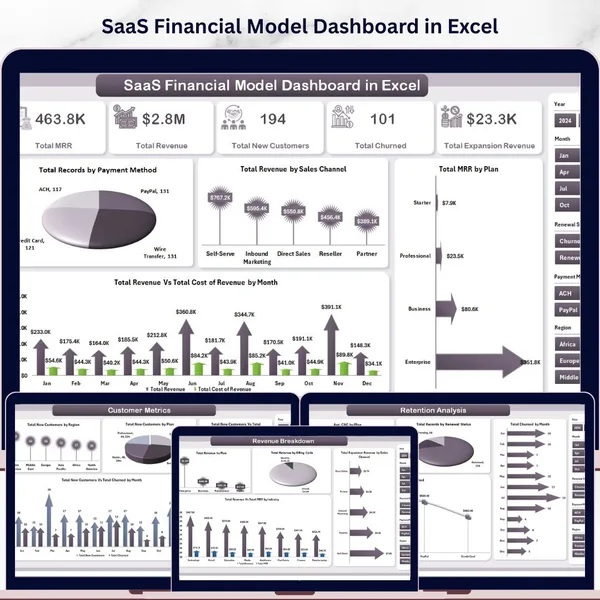
SaaS Financial Model Dashboard in Excel
MRR, churn, customer metrics and profitability across five dashboard pages.
View the pro template
PK is the founder of PK: An Excel Expert and NextGenTemplates.com and a corporate trainer in Excel, VBA and Power BI. Since 2020 he and his team have built Excel and Google Sheets tutorials and templates for business users.
Education only. Not financial, tax or investment advice.